Deep Reinforcement Learning for Dynamic Multichannel Access
PyTorch replication of Wang et al. (2018) "Deep Reinforcement Learning for Dynamic Multichannel Access." DQN vs. the analytical optimal policy on the round-robin switching case
Python · updated Sep 2026
From the repository
Deep Reinforcement Learning for Dynamic Multichannel Access
A from-scratch replication of Wang, Liu, Gomes & Krishnamachari, "Deep Reinforcement Learning for Dynamic Multichannel Access in Wireless Networks" (arXiv:1802.06958).
Motivation
Dynamic spectrum access is one of the core problems in cognitive radio. The standard approach in the literature assumes channels switch independently, but in real deployments (WSNs on 2.4 GHz, for example) channels are correlated: external interference from Wi-Fi, Bluetooth, and microwave ovens affects multiple channels at once. When channels are correlated, the joint system state lives in a space of configurations and is only partially observable, so classic MDP solutions fail. Wang et al. show that a Deep Q-Network can learn a near-optimal channel access policy in this setting without knowing the transition probabilities a-priori. This repository reproduces that result end-to-end, verifies it against the paper's analytical optimal policy (Theorem 1).
Problem Setup
A single secondary user shares spectrum with primary users across channels (fixed in the paper's experiments, not treated as a free parameter). This is a single-agent problem with one learning agent, one channel choice per time step. Multi-user variants are discussed by the authors as future work and are not implemented here.
Each channel is a two-state (good/bad) process. Unlike the classical Gilbert-Elliot model, channels are correlated with each other rather than switching independently, so the joint system state lives in a space of configurations (Section III).
Per-channel marginal view. Each channel is good or bad at each time slot. In the round-robin case these are not independent: the system has exactly one good channel, which holds its position with probability or advances by one slot with probability . The two-state diagram above describes how an individual channel's marginal state evolves, not the joint dynamics.
At each time step the agent picks exactly one channel, observes only whether that channel was good or bad, and gets (success i.e picked good channel) or (transmission failure i.e picked a bad channel). It never observes the other channels and never has access to the transition probabilities. That makes this a POMDP as the true joint state is never fully observed.
Section VII-B (this repo's case): single good channel, round-robin switching.
If channel is good at time , it stays good with probability , or the next channel in sequence becomes good instead with probability p. This is the simplest case of the paper's "fixed-pattern" switching (Section VI), where channels are grouped into subsets activated in a fixed sequence.
Section VI (optimal-policy baseline):
With probability , the switching order, and the initial subset known a-priori, the optimal policy (Theorem 1) is a simple threshold rule where if , stay on the current channel after a bad observation and advance after a good one, else if , the rule flips. This is the ground-truth upper bound to check the DQN against.
Section VII-A (state encoding):
The DQN's input state is the past M=N per-slot observation vectors concatenated together, each a length-N vector with at the selected channel if good, if bad, and everywhere else.
Methods Implemented
| Method | Description | Requires known dynamics? |
|---|---|---|
| Optimal policy (Theorem 1) | Closed-form policy for fixed-pattern switching | Yes |
| Whittle Index heuristic | MLE-estimated per-channel transition matrix + index policy | No (estimates it) |
| DQN | ReLU hidden layers, -greedy (), experience replay, Adam | No |
Architecture
- State: past actions + observations (input dim )
Methodology Notes
Three non-obvious issues surfaced during replication and materially affect the Fig. 4 numbers. They are recorded here because they would not be obvious from a casual read of the paper.
-
Discounted return's effective horizon. With =0.9, the sum of over is out of the effective horizon which is approximately of the discounted return comes from the first steps of a trajectory. Naive per-episode evaluation therefore measures cold-start transient rather than steady-state policy quality. We run
BURN_IN=200steps unscored before accumulating discounted reward overSCORE_STEPS=1000. -
Genie initialization for Theorem 1. The optimal policy requires knowing the initial active channel (Section VI). An earlier version of the evaluation initialized the policy to a fixed channel regardless of the environment's true initial state, which broke the policy's invariant. After its first bad observation, the policy would stay on a channel that was not the true good one. The final evaluation syncs the policy to the environment's true initial channel, matching Theorem 1's stated assumption.
-
Equal evaluation protocol across policies. DQN is averaged over training seeds eval trajectories ( samples); Optimal, Whittle, and Random are each averaged over eval trajectories. Ealier the DQN was reported with error bars but baselines were reported as single samples whihc produced misleading "DQN beats Optimal" readings.
Results
Round-robin switching (reproduces Fig. 4)
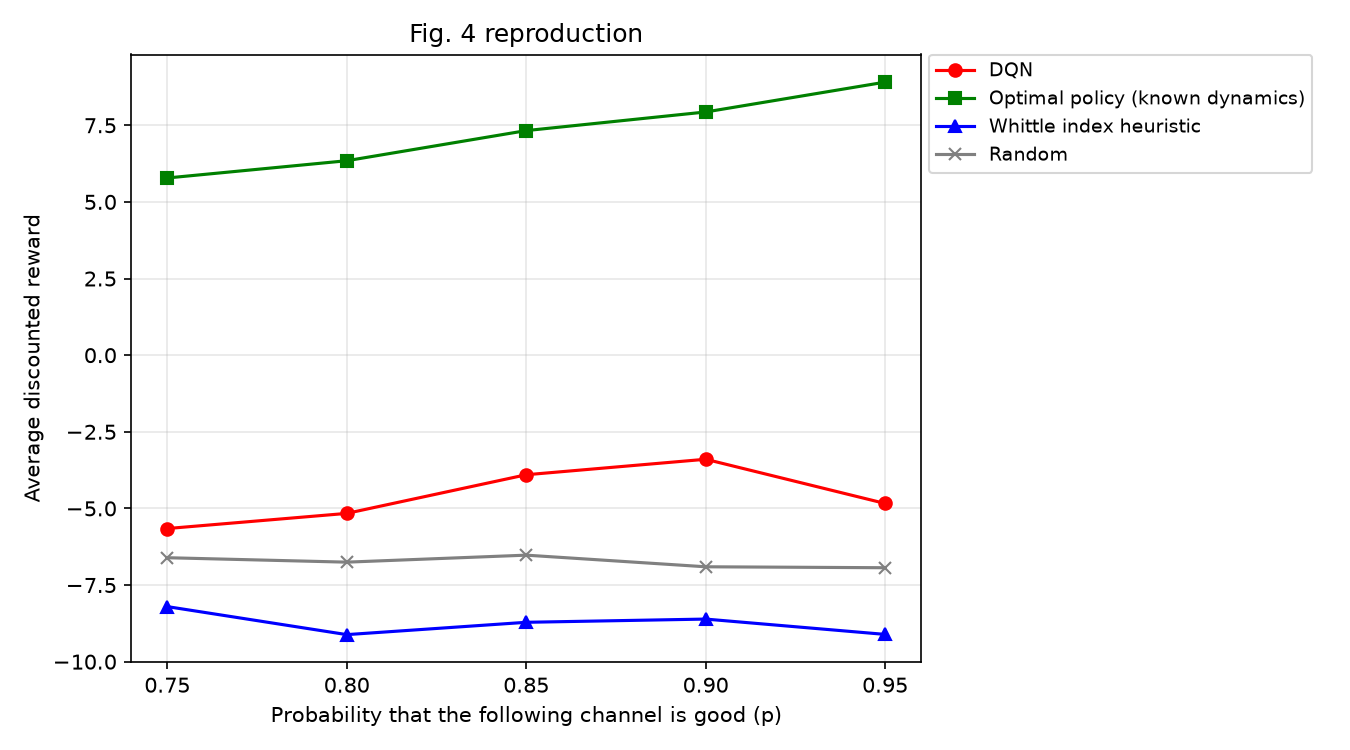
Initial run
When the DQN was underperforming due to smaller training steps and episodes.
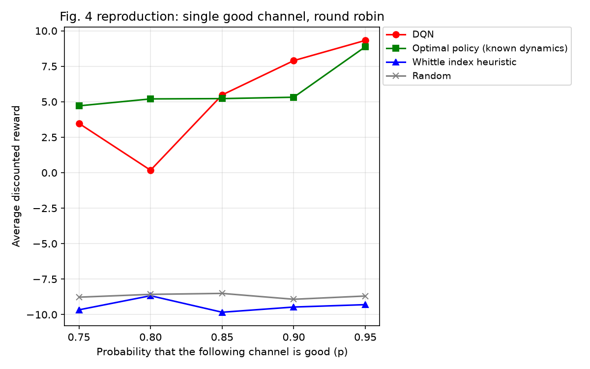
Second run
The result after increasing the training steps, but still not desireable output.
Latest run with more training episodes
After increasing training steps to 400k steps, a desireable and paper similar result was obtained.
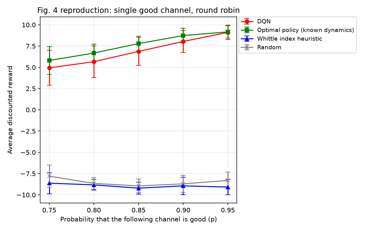
DQN tracks the shape of the Optimal policy across , but does not fully close the gap, and the size of that gap shrinks as increases. Results (mean std, discounted return over eval trajectories training seeds):
| p | DQN | Optimal | Whittle Index | Random |
|---|---|---|---|---|
| 0.75 | ||||
| 0.80 | ||||
| 0.85 | ||||
| 0.90 | ||||
| 0.95 |
At the completed values, DQN reaches of Optimal's discounted return at , rising to at . The gap narrows as increases. The paper reports that DQN achieves the same optimal performance as the optimal policy across all , the residual gap in this replication is its central discrepancy.
Whittle Index sits close to Random across all , and both sit far below DQN and Optimal. This is consistent with the paper's discussion of why an independent-channel heuristic cannot exploit the round-robin correlation.
Running
pip install -r requirements.txt

# Main Fig. 4 sweep (~3-4 hours).
python -m experiments.exp1_round_robin
References
- Wang, S., Liu, H., Gomes, P. H., & Krishnamachari, B. (2018). Deep reinforcement learning for dynamic multichannel access in Wireless Networks. IEEE Transactions on Cognitive Communications and Networking, 4(2), 257–265. https://doi.org/10.1109/tccn.2018.2809722 Also in (arXiv:1802.06958)